Forecasts by PHONIAC
Peter Lynch, UCD
Meteorology & Climate Centre,
Owen Lynch,
The
first computer weather forecasts were made in 1950, using the ENIAC (Electronic
Numerical Integrator and Computer). The ENIAC
forecasts led to operational numerical weather prediction within five years,
and paved the way for the remarkable advances in weather prediction and climate
modelling that have been made over the past half
century. The basis for the forecasts was the barotropic
vorticity equation (BVE). In the present study, we
describe the solution of the BVE on a mobile phone (cell-phone), and repeat one
of the ENIAC forecasts. We speculate on the possible applications of mobile
phones for micro-scale numerical weather prediction.
The ENIAC Integrations
The
ENIAC forecasts were described in a seminal paper by Jule
Charney, Ragnar Fjørtoft and John von Neumann (1950; referenced
below as CFvN). The story of this work was recounted
by George Platzman in his Victor P. Starr Memorial
Lecture (Platzman, 1979). The atmosphere was treated
as a single layer, represented by conditions at the 500 hPa
level, modelled by the BVE. This equation, expressing
the conservation of absolute vorticity following the
flow, gives the rate of change of the Laplacian of
height in terms of the advection. The tendency of the height field is obtained
by solving a Poisson equation with homogeneous boundary conditions. The height
field may then be advanced to the next time level. With a one hour time step,
this cycle is repeated 24 times for a one-day forecast.
The
initial data for the forecasts were prepared manually from standard operational
500 hPa analysis charts of the U.S. Weather Bureau, discretised to a grid of 19 by 16 points, with grid interval
of 736 km. Centred spatial finite differences and a
leapfrog time-scheme were used. The
boundary conditions for height were held
constant throughout each 24-hour integration. The forecast starting at 0300 UTC,
Dramatic growth in computing power
The
oft-cited paper in Tellus (CFvN) gives a complete account of the computational algorithm
and discusses four forecast cases. The ENIAC, which had been completed in 1945,
was the first programmable electronic digital computer ever built. It was a
gigantic machine, with 18,000 thermionic valves, filling
a large room and consuming 140 kW of power. Input and output was by means of
punch-cards. McCartney (1999) provides an absorbing account of the origins,
design, development and destiny of ENIAC.
Advances
in computer technology over the past half-century have been spectacular. The
increase in computing power is encapsulated in an empirical rule called
The principal designers of ENIAC were John Mauchly
and Presper Eckert. It is noteworthy that Mauchley’s interest in computers arose from his
desire to forecast the weather by calculation. The computer was originally
called the Electronic Numerical Integrator. A U.S. Army Colonel suggested
adding the words “and Computer” to give the catchy acronym ENIAC
(McCartney, 1999). This set a trend for naming computers: later machines
designed by Mauchly and Eckert were called EDVAC, BINAC
and UNIVAC. Computers based on John von Neumann’s design were called
JOHNNIAC and ILLIAC. Nicholas Metropolis of Los Alamos National Laboratory
named his version of this line MANIAC (Mathematical Analyzer, Numerator,
Integrator and Computer) in the hope of stemming the tide
of silly acronyms. But his was a vain hope: the first Australian computer was
called SILLIAC (
Recreating the Forecasts
Lynch
(2008) presented the results of repeating the ENIAC forecasts using a Matlab program eniac.m,
run on a laptop computer (a Sony Vaio, model
VGN-TX2XP). The main loop of the 24-hour forecast ran in about 30 ms. Given
that the original ENIAC integrations each took about one day, this time ratio -
about three million to one - indicates the dramatic increase in computing power
over the past half century. The program eniac.m
was converted from MatLab to a Java application, phoniac.jar,
for implementation on a mobile phone. Java Platform, Micro Edition (Java ME) is
a system for the development of software for small, resource-limited devices such
as cell phones. The program phoniac.jar
was tested on a PC using emulators for three different mobile phones. A basic
graphics routine was also written in Java. When working correctly, the program wasdownloaded onto a Nokia 6300 for execution.
Charney
et al. (1950) provided a full description of the solution algorithm for the BVE.
The programs eniac.m and phoniac.jar
were constructed following the original algorithm precisely, including the
specification of the boundary conditions and the Fourier transform solution
method for the Poisson equation. Hence, given initial data identical to that used
in CFvN, the recreated forecasts should be identical
to those made in 1950. Of course, the reanalyzed fields are not identical to those
originally used, and the verification analyses are also different. Nevertheless, the original and new results are very similar.
The
initial fields for the four ENIAC forecasts were valid for dates in January and
February, 1949. A retrospective global analysis of the atmosphere, covering
more than fifty years, has been undertaken by the National Centers for
Environmental Prediction (NCEP) and the
Fig.
2 shows the recreated forecast for 0300 UTC on January 6. The main features of the analysis (left
panel) and forecast (right panel) are in broad agreement with the originals in
Fig. 1. This forecast, run on the laptop computer with the program eniac.m, is
discussed in Lynch (2008). In Fig. 3 we show PHONIAC and the forecast for 0300
UTC,
In
CFvN it is noted that the computation time for a
24-hour forecast was about 24 hours, that is, the team could just keep pace
with the weather provided the ENIAC did not fail. This time included off-line
operations: reading, punching and interfiling of punch cards. PHONIAC executed
the main loop of the 24-hour forecast in less than one second. The main steps
in the solution algorithm are presented in Lynch (2008, Appendix B). For the
benefit of students, the MatLab and Java codes are
available on a web-site (http://maths.ucd.ie/~plynch/eniac/).
Maps of the four original and recreated forecasts
are also available there, along with miscellaneous supplementary material
relating to the ENIAC integrations.
Micro-scale forecasting
The computing power of
cell-phones is significant, and is growing rapidly. The Nokia 6300 runs at a
frequency of about 237 MHz, with one million instructions per second (MIPS) per
MHz. The phone supports “jazelle”, a
technology to execute Java byte-code in hardware, so that one instruction
translates into one floating point operation. Thus, we may estimate the peak speed
of PHONIAC to be 237 MFLOPS (million floating-point operations per second). The
CRAY-1, the first super-computer acquired by the European Centre for
Medium-Range Weather Forecasts (ECMWF) reached 160 MIPS. Making full use of the
vector features (which is feasible for meteorological
applications) the CRAY-1 peaked at about 250 MFLOPS. Thus, in terms of raw
computational power the CRAY-1 and
the Nokia 6300 are in the same league. The CRAY-1 used some 115KW, comparable
to ENIAC; the Nokia 6300 uses about 1.5W under a full load.
The
graphics capabilities of modern mobile phones are also impressive. They provide
a basis for local processing of meteorological data. For example, selected
output from the Met Office 4 km
(http://www.metoffice.gov.uk/research/nwp/numerical/operational/)
could be acquired with a high time-frequency and statistically or dynamically
downscaled to sub-kilometre resolution. Combining
this with GPS data and high-resolution topographical data, local adaptation of
the flow could be simulated. One
could imagine a yachtsman modelling local eddies
during a race in the
Acknowledgement
The
assistance of Chi-Fan Shih in acquiring the NCEP/NCAR reanalysis data is
gratefully acknowledged. The java function
atan2
uses code written by Paulo Costa. We thank Hendrik
Hoffman, UCD, for advice on the comparative power of PHONIAC and Cray-1.
References
Charney, J. G., R. Fjørtoft
and J. von Neumann, 1950: Numerical
Integration of the Barotropic Vorticity
Equation. Tellus,
2, 237-254.
Kistler, R. et al.,
2001: The NCEP-NCAR 50-Year Reanalysis: Monthly Means, CD-ROM and
Documentation. Bull. Amer. Met. Soc., 82, 247-268.
Lynch,
Peter, 2008: The ENIAC forecasts: a recreation. Bull. Amer.
Met. Soc., 89, 45-55.
McCartney,
Scott, 1999: ENIAC: The Triumphs and Tragedies
of the World's First Computer.
Platzman, G. W., 1979:
The ENIAC computations of 1950 - gateway to numerical weather prediction. Bull. Amer. Met. Soc., 60, 302-312.
Figures
`
Figure
1. The ENIAC forecast starting at 0300 UTC,
Figure
2. Reconstruction of the ENIAC 24-hour forecast starting at 0300 UTC,
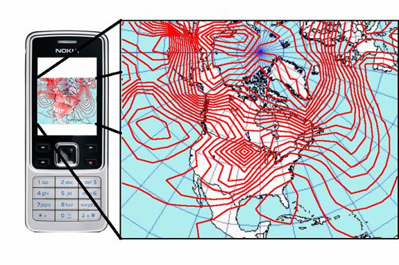
Figure
3. The Nokia 6300, dubbed PHONIAC (left) and the forecast for 0300 UTC,
Contact
details
|
Peter
Lynch UCD
Meteorology & Climate Centre School
of Mathematical Sciences Belfield,
E-mail:
Peter.Lynch (at) ucd.ie Web:
http://maths.ucd.ie/~plynch |
Owen
Lynch IBM
Ireland Damaston
Industrial Estate Mullhuddart,
Email:
lynchowe
(at) ie.ibm.com |